Young & Kot Engineering Research

Why Do Antennas Radiate?

by John Kot

I'd like to welcome you to the first of an occasional blog series on antennas and electromagnetism with a quote from my favourite book on the subject, "Principles of Electrodynamics" by Melvin Schwartz: "Electromagnetic theory is beautiful!" And it is beautiful, but that beauty can sometimes be veiled behind a lot of lengthy mathematics. So, the aim of this blog series is to share with you things that I have come across in a long career as an engineer working on antennas and waveguides which have helped me to understand the beautiful physics behind the mathematics. Mostly, we'll try to avoid any calculus, and stick mainly to physical arguments and discussions about geometry. With that said, let's get on with it!

First off, we'll look at the most basic question of all: how does an electric charge radiate?

EM radiation is an amazing thing. Electric charges, jiggling about somewhere out past the star Arcturus, can somehow cause current to flow in a radio telescope on Earth - currents which are tiny, but large enough for astronomers to amplify and record, and make radio maps of outer space. Currents on an antenna onboard a satellite forty thousand kilometres from Earth make signals flow in a receiver on your roof and allow you to watch TV shows. When you think about it like that, it seems almost impossible, and yet, that's what we measure. So, how does that happen? Of course, the correct answer is, "Solve Maxwell's equations and the solution will give you the answer." But, instead, let's just think about simple electrostatics, a bit of geometry, and the idea that nothing travels faster than the speed of light, and we'll find that, with these basic tools, we can get surprisingly far!

First of all, when do electric charges radiate? Einstein showed [1] that there is no essential difference between a stationary electric charge and a charge moving with constant velocity. You can always consult an observer moving along with the charge and they will report that they measure a static electric field filling space. So, if stationary charges do not radiate electromagnetic waves, then neither do charges in steady motion. Radiation must be associated with accelerated electric charges. Or, if you want to think in terms of electric current, a charge moving with uniform velocity is equivalent to a constant current. Therefore, it must be time-varying electric currents that act as a source for electromagnetic radiation.

As I said, you can find the EM field generated by an accelerated charge by solving Maxwell’s equations, but there is a more intuitive approach that comes from a simple geometrical argument plus a tiny bit of relativity (that the speed of light is a universal constant, and information cannot travel faster than that). This argument was first thought up by the Irish physicist Joseph Larmor. This is our thought experiment: the source of the radiation is a charge moving with uniform velocity $v_0$, which changes its velocity to a different uniform velocity $v_1$ by a brief, constant acceleration a over a short time $\Delta t$. The acceleration is uniform and so is given by the final velocity minus the initial velocity, divided by $\Delta t$:

$$a=\frac{dv}{dt}=\frac{v_1-v_0}{\Delta t}$$

Thanks to Einstein, we don’t lose generality by assuming that $v_1=0$, i.e., that the charge was initially moving with uniform velocity and then comes to rest. To make the equations simple, we assume that the charge is moving along the x-axis, and comes to rest at $x=0$, at time $t=0$. We measure the electric field at a distance $R$ from the origin, at an angle $\theta$ from the x-axis, as shown in Figure 1 below.

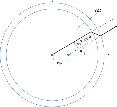
According to relativity, the information that the charge has come to rest at $t=0$ propagates outwards into space at the speed of light, $c$. At a later time, $t=T$, we can divide the world into three regions. At a distance $R$ greater than $c \times T$, the information that the charge has stopped moving hasn't yet reached this region, so outside this sphere the field must look like the field of the original moving charge, i.e., the field of a charge in uniform motion, located at $x=v_0 \times T$. Similarly, in the sphere $R<c\left(T - \Delta t \right)$ the information that the charge has stopped has already reached these points, and so the field is that of the stationary charge at the origin. In the space between these two spheres is the region influenced by the accelerated charge, where the interesting things happen. Let's draw the field in terms of electric field lines, as shown in Figure 1 above, recognizing that these “lines” are just a way of representing the force experienced by an infinitesimal test charge, i.e., they are simply a convenient means of visualizing the continuous field in space.

Because the electric field is continuous in a charge-free region, the field lines must be continuous as they pass through the region between the spheres, $cT\geq R\geq c\left(T- \Delta t \right)$, so the field lines have a “kink” in them. Outside this narrow region, the field is purely radial but, between the spheres, the field has both a transverse component $E_t$ and a radial component $E_r$. By simple geometry, the ratio of the transverse and radial components is:

$$\frac{E_t}{E_r}=\frac{v_0T\sin{\left(\theta\right)}}{c\Delta t}$$

To express this in more convenient terms, we note that:

$$R=c T;\ \ \ \ \ \ v_0 = a \Delta t$$

Substituting these expressions into the equation for $\frac{E_t}{E_r}$ we get:

$$\frac{E_t}{E_r}=a\Delta t\frac{R}{c}\sin{\left(\theta\right)}\frac{1}{c \Delta t}=\frac{a R\sin{\left(\theta\right)}}{c^2}$$

Now, $E_r$ is just the E-field of a static charge, so we know this from electrostatics:

$$E_r=\frac{q}{4\pi\varepsilon_0R^2}$$

So, we can immediately write down a final expression for the transverse field $E_t$:

$$E_t=\frac{q}{4\pi\varepsilon_0c^2}\frac{a\sin{\left(\theta\right)}}{R}$$

This transverse field is the radiation we are looking for, so we've solved the problem of EM radiation without any calculus at all! Not bad! But how do we know that this the transverse field is the radiation field? Well, the transverse field falls off like $R^{-1}$, while the radial field falls off like $R^{-2}$. In other words, if we double the distance $R$, then $E_t$ gets smaller by a factor 2, while $E_r$ gets smaller by a factor 4. What is the physical significance of this difference? It becomes clear when we think of the energy carried by the field.

The energy is proportional to $\left|E\right|^2$ so let's calculate the total amount of energy $U$ carried by the transverse field through a sphere of radius $R$. If we double $R$, then $E_t$ gets smaller by a factor 2, so $\left|E_t\right|^2$ gets smaller by a factor 4. But, the area of the sphere will get larger by a factor 4, so the total amount of energy summed up over the sphere will stay the same. Expressing this mathematically:

$$U\propto\left(\frac{qa}{4\pi\varepsilon_0c^2}\right)^2\int_{0}^{2\pi}d\varphi\int_{0}^{\pi}{R^2\sin{\left(\theta\right)}}\frac{\sin^2{\theta}}{R^2}d\theta=\left(\frac{qa}{4\pi\varepsilon_0c^2}\right)^2\frac{8\pi}{3}$$

Okay, I said there wasn't going to be any calculus. Well, there won't be any more calculus!

What this means is that, however large we make $R$, the total amount of radiation will stay constant! So $E_t$ is a radiation field carrying energy all the way to infinity. Of course, the energy is spread out very thinly over a large area, so the energy density is very small. That's why the radio telescope dish is large - to collect enough energy.

The other thing to note is the strength of the field is proportional to $\sin{\left(\theta\right)}$ from the direction of the velocity. In other words, there is no radiation in that direction.

In an antenna, it is easier to think about currents rather than charges. We can do this easily by writing the electric current $I$ as the charge times the velocity:

$$I=qv$$

Then

$$q a=q\frac{dv}{dt}=\frac{d\left(qv\right)}{dt}=\frac{dI}{dt}$$

Using this, the expression for the radiated field in terms of current is:

$$E_t=\frac{1}{4\pi\varepsilon_0c^2}\left(\frac{dI}{dt}\right)\frac{\sin{\left(\theta\right)}}{R}$$

The main results are that the radiated field is proportional to the rate of change of the current, and no energy is radiated along the direction of the current.

We have slightly glossed-over the fact that, in the inner and outer spherical regions, the observers who measure a static field are moving with respect to each other. In fact, a stationary observer in one frame will measure a slightly different field from the moving observer. This difference is the subject of Einstein's famous 1905 paper [1] where he shows that the difference seen by the two observers is what gives rise to the magnetic field.

References

[1]: Einstein, Albert (1923). "On the Electrodynamics of Moving Bodies". (English translation of the original 1905 paper in German) The Principle of Relativity. Translated by George Barker Jeffery; Wilfrid Perrett. London: Methuen and Company, Ltd.